All of It
 |
Contents |
For electromagnetism all you need to know is what happens when you have + or – charges, what happens when they get close and what happens when they move. That’s it! For all of non-quantum EM there are only 5 formulas you need. The 4 Maxwell Equations and the Lorentz equation describe all of electricity, magnetism, light, sound, radiation, actually most of physics:
(1) 
(2) 
(3) 
(4) 
(5) 
How bad can a topic be if you can describe it all with just 5 equations, you could probably fit them all on the back of a beermat. Now that you’ve seen the conclusion we can go to the beginning and read the whole story in detail. Unless you’re doing a university course you can get away with not knowing exactly what the equation mean or do, but this site will explain them later, first lets get back to basics.
The Basics
Charge comes in 2 types, positive and negative and is measured in Coulombs (C). If you have a charge on its own it emits a field in all directions. The field from a charge is represented by E as in E-lectricity. If you put another charge in the field it experiences a force. Like charges repel and unlike charges attract. The bigger the charge the stronger the force and the further away the charges the weaker the force, exactly what you’d expect. This relationship can be represented by Coulombs Law;
![\[F=\frac{1}{4\pi\epsilon_0}\frac{q_1q_2}{r^2}\]](https://physicsforidiots.com/wp/wp-content/ql-cache/quicklatex.com-66b313d86d4f9c40d2e1f5b540cb677b_l3.png "Rendered by QuickLaTeX.com")
and
![\[E=\frac{1}{4\pi\epsilon_0}\frac{q_1}{r^2}\]](https://physicsforidiots.com/wp/wp-content/ql-cache/quicklatex.com-dda60162bc43fed2108dad882fa9083a_l3.png "Rendered by QuickLaTeX.com")
The  ‘s are the two charges and
  is the distance between them squared. The other bit is just a constant which roughly equals 9000000000. (The exact derivation of this law can be found here). From these you can see that the force is just the field times by whatever charge you put in,
  . Using this you can work out the field or force between particles or atoms or anything with charge provided they’re not moving. Once you start a charge moving other things happen.
Stuff Moving
As soon as a charge starts to move it produces another field. The new field is magnetism and is represented by B as in B-magmatism?
The reason it’s B is simply that it was the second thing in an alphabetical list:
- Electromagnetic vector potential: A
- Magnetic induction: B
- Total electric current: C
- Electric displacement: D
- Electromotive force: E
- Mechanical force: F
- Velocity at a point: G
- Magnetic intensity: H
(This also explains where H comes from for those interested).
So now your particle or atom or whatever has 2 fields coming out. The full equation to describe how both fields act on a particle is
![\[F=q(E+v\times B)\]](https://physicsforidiots.com/wp/wp-content/ql-cache/quicklatex.com-a4859d023e331765486615b5aa46343e_l3.png "Rendered by QuickLaTeX.com")
which is known as the Lorentz force. The  symbol does not signify multiplication, in this context it means Cross-Product. It’s basically a short way of writing “
 times
times  times the sine of the angle between”. This is because the field pushes at 90° to which ever direction its pointing AND which ever direction you are moving in. Now unless you’re doing EM past A-level you can forget all about the directions and angles and just write
![\[F=q(E+vB)\]](https://physicsforidiots.com/wp/wp-content/ql-cache/quicklatex.com-406cf5b2d3f017c3cd6fcddfb64b5c7a_l3.png "Rendered by QuickLaTeX.com")
If we expand out the above expression we have
![\[F=qe+q(v\times B)\]](https://physicsforidiots.com/wp/wp-content/ql-cache/quicklatex.com-7796a47b68015864b68b41779f0d0b85_l3.png "Rendered by QuickLaTeX.com")
But we can already describe one of these bits,  is just Coulombs Law. Also, at A-level or below the situation will probably be simplified so you only have to consider the
  and fields separately. So you will probably only have to use one of the following two formulas,
![\[F=qE\]](https://physicsforidiots.com/wp/wp-content/ql-cache/quicklatex.com-9dea8fa7476d245890675b751b1ef518_l3.png "Rendered by QuickLaTeX.com")
![\[F=qvB\]](https://physicsforidiots.com/wp/wp-content/ql-cache/quicklatex.com-9fa53d4752d348dc6c1d8df0615863c1_l3.png "Rendered by QuickLaTeX.com")
Obviously  is the force and is charge, and are the two fields previously described and is the velocity of the moving charge. The electric field is measured in the SI units of Newtons per coulomb (
 ) or, equivalently, volts per meter (
 ). The magnetic field has the SI units of Teslas (T), equivalent to Webers per square meter (
 ) or volt seconds per square meter (
 )
)
Circuits
Now I’m not a big fan of circuits, never have been, now hopefully I’ll be professional enough that my disliking of them won’t come across in this section but if it does I apologise in advance. If I really start to struggle with my hate I may have to call in a second writer
A circuits is basically just a series of moving charges with the occasional object or device in the way that affects the flow. Now when I say the electrons are moving around most people will think that their speeding around at close to the speed of light, but this is wrong. The actual electrons are moving EXTREMELY slowly, it’s the wave that travels fast. As stated above like charges repel, so put one electron next to another and they will move apart. With a current in a wire you basically have a tube of electrons and you’re adding one to one of the ends, this causes the next electron to move down which in turn pushed the next one and so on. So you have a Mexican wave like effect that moves quickly, but the electrons themselves are only moving slowly.
Circuits usually contain all sorts of different objects and devices depending on what they’re for, and depending on how you set them all up in the circuit depends how you do all of you calculations.
Which is Which?
If you set up all your component in a closed loop like so
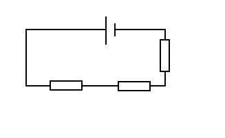
then we say that all the components are in Series. If you set them up with branching paths like so

then we say that the components are in Parallel. You can also make circuits that are a mixture of series and parallel section like so

Amps, Volts and Ohms (Oh my!)
We call the moving charges a Current, and it is measured in the SI unit of Amps (A). Amps are equivalent to the amount of charge passed in a certain time, so 2 coulombs in 6 seconds will be equivalent to 0.3A. This, like most things in physics can be expressed in a nice formula for you to learn
![\[I=\frac{Q}{t}\]](https://physicsforidiots.com/wp/wp-content/ql-cache/quicklatex.com-f1fc11449243ff24d70ac987efec487f_l3.png "Rendered by QuickLaTeX.com")
Another important idea in circuits is Voltage or Potential Difference. Volts are basically the difference in the Electric potential at two different points. The electric potential between 2 points is given as
![\[V=V_b - V_a = \int_b^aE.dl\]](https://physicsforidiots.com/wp/wp-content/ql-cache/quicklatex.com-0035b17b288e8758ba223f280fd1370a_l3.png "Rendered by QuickLaTeX.com")
where  is the distance between
  and
and  . It’s basically field times distance.
Another important idea when it comes to circuits is resistance. Resistance is basically a measure of how much resistance opposes an electric current. Almost all objects or devices in a circuit cause resistance and to calculating the total resistance in a circuit you use one or more of these rules
![\[R_{series}=R_1 + R_2 + R_3 + R_4 + \bdots\]](https://physicsforidiots.com/wp/wp-content/ql-cache/quicklatex.com-a81ef2045addd71474e2cb4a55f3cbb3_l3.png "Rendered by QuickLaTeX.com")
![\[\frac{1}{R_{parallel}}=\frac{1}{R_1} +\frac{1}{R_2} +\frac{1}{R_3} +\frac{1}{R_4} + \bdots\]](https://physicsforidiots.com/wp/wp-content/ql-cache/quicklatex.com-18116a1d3f9937f152e12bac487ee1a2_l3.png "Rendered by QuickLaTeX.com")
One of the most important and fundamental equations in circuits is Ohm’s law, and it relates current, voltage and resistance.
![\[V=IR\]](https://physicsforidiots.com/wp/wp-content/ql-cache/quicklatex.com-93f15587dbfd868135bd7d85a3472c6e_l3.png "Rendered by QuickLaTeX.com")
The Deep End
This is it. Classical EM goes no deeper than this. These 4 are the fundamental equation for ALL fields in EM. They may take a bit to get your head around but once you do it should all make sense, sort of.
![\[\oint E.dA=\frac{Q_{inside}}{\epsilon_0}\]](https://physicsforidiots.com/wp/wp-content/ql-cache/quicklatex.com-e7351cc5c826c68e1b69ea300365ae81_l3.png "Rendered by QuickLaTeX.com")
![\[\oint B.dA=0\]](https://physicsforidiots.com/wp/wp-content/ql-cache/quicklatex.com-b1d923f8f2fafe41d5dabb08016b435e_l3.png "Rendered by QuickLaTeX.com")
![\[\oint E.dl=-\int\frac{\partial B}{\partial t}.dA\]](https://physicsforidiots.com/wp/wp-content/ql-cache/quicklatex.com-adf3c1248d8075f01f257bb7f70fc4ad_l3.png "Rendered by QuickLaTeX.com")
![\[\oint B.dl=\mu_0I+\mu_0\epsilon_0\int\frac{\partial E}{\partial t}.dA\]](https://physicsforidiots.com/wp/wp-content/ql-cache/quicklatex.com-49647b174f57fa6699e3384ccc3c2481_l3.png "Rendered by QuickLaTeX.com")
If you don’t know about integration and differentiation I suggest you head over to the Integration section or the Differentiation section, I’ll try to explain it here but I’ll mainly be focusing on the physics.
Gauss’ Law
Ok then first up we have Gauss’ Law.
This says that the integral of the Electric field, , through a closed area  is equal to the total charge inside of the area,
  divided by
  . is a constant called The Permittivity of Free Space and shows up all over physics along with
  which is The Permeability of Free Space. What this equation means is you can take ANY closed surface you like and find the field going through, provided you can do the maths. Usually you can’t. However there are a number of cases when its nice and easy. Cases when the field is coming straight out through the surface evenly. The cases are
- A Spherical surface around a point or sphere
- A Cylindrical surface around an infinite wire
- A Regular surface over a section of an infinite plane
I admit these sound vague and abstract so I will demonstrate with the aid of a diagram.
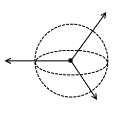
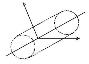
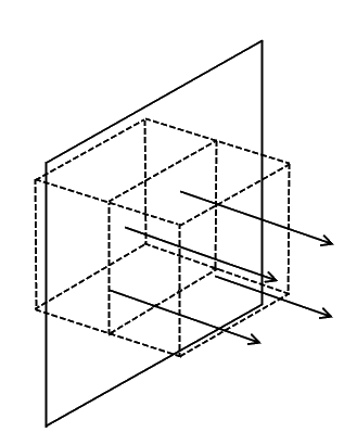
These are the Gaussian surfaces. Basically with these surfaces all you’re trying to do is make life easier. You just make sure that the surface is always the same distance from the charge source and that the field is always going through at 90 degrees. You can then work out the integral with your eyes closed its that easy. The left hand side of Gauss’ law becomes E times the surface of the shape you chose.
- A Spherical surface becomes
 , where
  is the radius of the sphere.
 - A Cylindrical surface becomes
 , where and are the length and radius of the cylinder.
 - A Regular surface becomes
 , where
  is the Area above and below the infinite surface (you need the factor of 2 as the field goes above and below the surface at 90 degree).
So Gauss’ law for a sphere becomes
![\[4\pi r^2E=\frac{Q_{inside}}{\epsilon_0}\]](https://physicsforidiots.com/wp/wp-content/ql-cache/quicklatex.com-e2d7a4d1252543b8228bdcdb4e8c7a7d_l3.png "Rendered by QuickLaTeX.com")
![\[E=\frac{1}{4\pi\{epsilon_0}\frac{Q_{inside}}{r^2}\]](https://physicsforidiots.com/wp/wp-content/ql-cache/quicklatex.com-f6628cfc7794548de213a7c896e7b0aa_l3.png "Rendered by QuickLaTeX.com")
Which was introduces earlier as Coulombs Law, now you know where it came from. Gauss’ Law for an infinite line of charge is just
![\[2\pi r l E=\frac{\lambda l}{\epsilon_0}\]](https://physicsforidiots.com/wp/wp-content/ql-cache/quicklatex.com-2e4f9e51641102bed93affd344f37dd7_l3.png "Rendered by QuickLaTeX.com")
![\[E=\frac{\lambda}{2\pi{\epsilon_0}r}\]](https://physicsforidiots.com/wp/wp-content/ql-cache/quicklatex.com-aa040719a7c0f62f175c6d8708ca5d4a_l3.png "Rendered by QuickLaTeX.com")
Now in this something new has been introduced,  . If you have an infinite line of charge then the total charge on it is infinite and there is no way of knowing how much of that infinite charge you would have inside your gaussian surface. That’s where comes in, its a value of charge per unit length, so if =4Cm
 and you have 5 metres then the charge is just 20C. That’s all is, just a value of charge.
For an infinite surface gauss’ law becomes
![\[E=\frac{\sigma}{2{\epsilon_0}}\]](https://physicsforidiots.com/wp/wp-content/ql-cache/quicklatex.com-0fbebc10a7021c530ddfd4ab21070555_l3.png "Rendered by QuickLaTeX.com")
Once again a new symbol has been added but its just like the one before.  is just the charge per unit area, so if =5Cm
 and you have a 100m
 area the total charge is 500C.
Charged Ring
Lets say you’ve got a charged ring and you need to know the field produced from it. Once again we’ll be employing one of the most important tools in physics, making stuff easier. Firstly we’ll only look at the field along the axis of the ring, otherwise things just get too complicated and it’s not worth the effort. Now lets just take a very small part of the ring and say that it’s a sphere. This isn’t really true, but the smaller we make the section the more we can make it resemble a point charge. So you have something like this
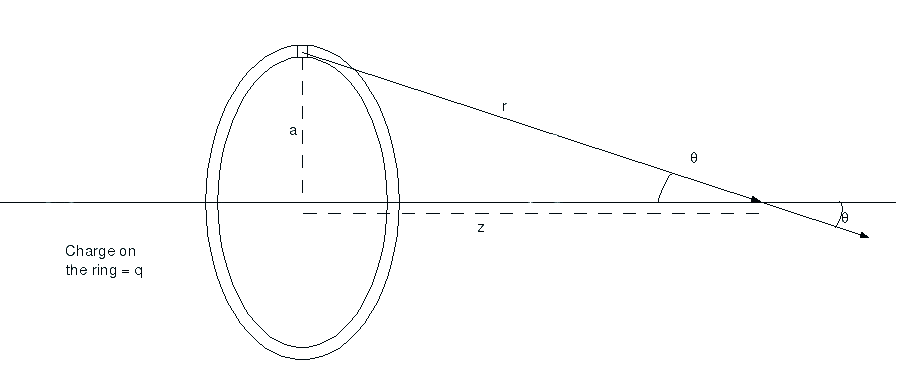
You want to find the field at a point  along the axis from the ring of total charge and radius . The little square section at the top, that’s the bit that you assume is a charged sphere. Now we don’t know how much charge is in that little section as you can make it any size you want so we just call the charge
  , a small amount of . So we now have
![\[E=\frac{1}{4\pi\epsilon_0}\frac{dq}{r^2}\]](https://physicsforidiots.com/wp/wp-content/ql-cache/quicklatex.com-7ad1f207332400a9bd61dce300342205_l3.png "Rendered by QuickLaTeX.com")
Now if you think about it, every bit of the ring above the axis pushing down will have an equal bit below the axis pushing up. It’ll also be the same for left and right and all other parts of the ring. So all the force from the ring will only be acting along the axis. To work out only this bit we need to use some trig. We need to times the field by  to get the axial component.
![\[E=\frac{1}{4\pi\epsilon_0}\frac{dq}{r^2}\cos\theta\]](https://physicsforidiots.com/wp/wp-content/ql-cache/quicklatex.com-f3c7ab429f1b7892dcc7a465fa0b26d0_l3.png "Rendered by QuickLaTeX.com")
As you may or may not know can also be described (using SOH CAH TOA) by the following relationship for our situation
![\[\cos\theta=\frac{z}{r}\]](https://physicsforidiots.com/wp/wp-content/ql-cache/quicklatex.com-e5b86813191be6cca9051227974bc4ba_l3.png "Rendered by QuickLaTeX.com")
As is the adjacent side and is the hypotenuse. So now we have
![\[E=\frac{1}{4\pi\epsilon_0}\frac{zdq}{r^3}\]](https://physicsforidiots.com/wp/wp-content/ql-cache/quicklatex.com-26740302c76bdd187c06316eed67659d_l3.png "Rendered by QuickLaTeX.com")
However we may not know what is. We do know the radius of the disk, , and the distance we are from the disk, . Using a bit of the old Pythagoras we can rewrite in terms of and
![\[r=\sqrt{z^2+a^2}\]](https://physicsforidiots.com/wp/wp-content/ql-cache/quicklatex.com-174e2a961ce0dde8007d87da9d32ab05_l3.png "Rendered by QuickLaTeX.com")
So now our equation looks like this
![\[E=E=\frac{1}{4\pi\epsilon_0}\frac{zdq}{(z^2+a^2)^{3/2}}\]](https://physicsforidiots.com/wp/wp-content/ql-cache/quicklatex.com-083a88d7e5d9667a2d0777a010600649_l3.png "Rendered by QuickLaTeX.com")
Now we want to get rid of that , so we integrate
![\[E=\frac{1}{4\pi\epsilon_0}\int\frac{z}{(z^2+a^2)^{3/2}}dq\]](https://physicsforidiots.com/wp/wp-content/ql-cache/quicklatex.com-81fd20b997838de179adfcfc3ae64ea1_l3.png "Rendered by QuickLaTeX.com")
Now we know from the diagram at the start that the total charge on the disk is , so if we add up all the little bits of the total should be , so the integral is just .
![\[E=\frac{1}{4\pi\epsilon_0}\frac{zq}{(z^2+a^2)^{3/2}}\]](https://physicsforidiots.com/wp/wp-content/ql-cache/quicklatex.com-02aa6e8af87fb5e03470ae1a56f32185_l3.png "Rendered by QuickLaTeX.com")
So there you have it, the field from a charged disk. All you need is the field from a point and some trig knowledge and you can work it out. I could have just given you the final solution, but this way you can see where it came from and then if you forget it you may be able to work it out from first principles like above.
Gauss’ Law for Magnetism
This one is nice and easy but has some big implications. Gauss’ Law for Magnetism is
Its like the ordinary gauss’ law in that it describes a field, this time its the magnetic field, . It says that the integral of B over a closed surface,  is zero. Nothing. Every field line that goes out of the surface has an equivalent that goes in. There is no overall field. This means that its impossible to get sources of Magnetic field. Whereas electrons and protons are origins of field, from which field lines diverge from or converge to, there is no magnetic analogue. Magnetic field lines are always closed loops, no start, no end. This of course hasn’t stopped people from preparing in case we do find a magnetic monopole.
This equation may seem nice, and it is, but it is utterly useless on its own. Usually a 0 result in physics is quite important, it means something special might be happening, here it shows magnetic monopoles don’t exist.
Faradays Law
Now things are getting more complex, here we have Faradays law,
I’ll walk you through each bit to show you what it actually means. First we have the left hand side which is easy. Its just like Gauss’ law only the integral is over a different thing. Instead of finding the total field through a surface, , we are now finding the total field around a closed loop  . That’s all that’s different with the left hand side, no more surfaces, just closed loops. Now on to the right hand side. First up we have a minus, noting complicated about that. Why its there will be explained later. Next we have another integral, and this one looks horrible. The
  symbol basically means a small change. So
  is a change in , and
  is a change in
  , where is time. The whole
  is the rate of change of , its how much is changing () in a given time (). And that is being integrated over an area . is the area inside the closed loop , if you draw some random squiggly thing making sure that the line doesn’t cross itself and that it joins itself then the length around the line is your and the area inside the line is your . Simple yes? So the total around a loop is just equal to the minus of the changing through the loop.
What happens if there is no ? Well there is no so is zero, which makes the integral 0, so no . What happens if you have a constant ? Well again is 0. So is zero, which makes the integral 0, so again no . You can only induce an field from a changing field.
The importance of the minus sign comes from the fact that fields create fields and fields create fields (As shown in Faraday’s and Ampere’s Laws). If the minus wasn’t there then the fields would just keep building and building eventually giving infinite energy, and that is not allowed!
Ampère-Maxwell Law
The last of Maxwell’s Equations is the Ampere-Maxwell law. Just like the first two laws were similar so are the last two, there is a pattern to them in this order that can make them easier to remember. over an area, over an area, around a loop and now finally around a loop. The equation is
Left hand side, easy, integral of B around a closed loop. Right hand side, not so easy. First lets ignore the  bit, I’ll come back to that. Other than the
  , its very similar to Faradays law. You have another changing field integrated over an area, but this time its . This time though instead of multiplying by minus 1 you’re multiplying by
  . Once again these are two very important values in physics, alone and combined. They are at the very heart of EM. So your magnetic field around a loop is just equal to the changing E field going through it times by , but then you have to add on a bit. This is the bit. This is just the current going round the loop times by , this is because, as said in Stuff Moving, if you have a moving charge i.e. a current, then you get a magnetic field. So you have to add the two bits together. There, done.
Another Form of the Deep End
As well as writing Maxwell’s equations above, in what is called integral form, you can also write them in differential form like so
![\[\nabla\cdot E=\frac{\rho}{\epsilon_0}\]](https://physicsforidiots.com/wp/wp-content/ql-cache/quicklatex.com-81a07dcc887fe21f3267358fbf53c159_l3.png "Rendered by QuickLaTeX.com")
![\[\nabla\cdot B=0\]](https://physicsforidiots.com/wp/wp-content/ql-cache/quicklatex.com-caeec9fb39538a859ad26e84421d7242_l3.png "Rendered by QuickLaTeX.com")
![\[\nabla \times E=-\frac{\partial B}{\partial t}\]](https://physicsforidiots.com/wp/wp-content/ql-cache/quicklatex.com-7e44ef899d200cb51fa9b2a17b82eb97_l3.png "Rendered by QuickLaTeX.com")
![\[\nabla \times B=\mu_0\left(J+\epsilon_0\frac{\partial E}{\partial t}\right)\]](https://physicsforidiots.com/wp/wp-content/ql-cache/quicklatex.com-cc0818c33ba5d09a4348dc0846860a8e_l3.png "Rendered by QuickLaTeX.com")
Yet Another Form of the Deep End
Writing Maxwell’s equations in one of the above two forms is really a simplification. Both the integral form and the differential form are vector equations and they save you having to write out the full 8 Maxwell equations for the and fields in all three dimensions.
[su_spoiler title=”8 ‘Original’ Maxwell Equations” style=”fancy”]
![\[\frac{\partial E_x}{\partial x}+\frac{\partial E_y}{\partial y}+\frac{\partial E_z}{\partial z}=\frac{\rho}{\epsilon_0}\]](https://physicsforidiots.com/wp/wp-content/ql-cache/quicklatex.com-0fe4708add78cb67574e6f3315d5fcab_l3.png "Rendered by QuickLaTeX.com")
![\[\frac{\partial B_x}{\partial x}+\frac{\partial B_y}{\partial y}+\frac{\partial B_z}{\partial z}=0\]](https://physicsforidiots.com/wp/wp-content/ql-cache/quicklatex.com-8d7c18277dd3be7485057bea0e639784_l3.png "Rendered by QuickLaTeX.com")
![\[-\frac{\partial B_x}{\partial t}=\frac{\partial E_z}{\partial y}-\frac{\partial E_y}{\partial z}\]](https://physicsforidiots.com/wp/wp-content/ql-cache/quicklatex.com-1fe44894674317aab6b723921d19d763_l3.png "Rendered by QuickLaTeX.com")
![\[-\frac{\partial B_y}{\partial t}=\frac{\partial E_x}{\partial z}-\frac{\partial E_z}{\partial x}\]](https://physicsforidiots.com/wp/wp-content/ql-cache/quicklatex.com-353b8c3330ba4faace45b7ce3ecaaf54_l3.png "Rendered by QuickLaTeX.com")
![\[-\frac{\partial B_z}{\partial t}=\frac{\partial E_y}{\partial x}-\frac{\partial E_x}{\partial y}\]](https://physicsforidiots.com/wp/wp-content/ql-cache/quicklatex.com-24094835269b709f2043f43483c706b5_l3.png "Rendered by QuickLaTeX.com")
![\[\mu_0\left(J_x+\epsilon_0\frac{\partial E_x}{\partial t}\right)=\frac{\partial B_z}{\partial y}-\frac{\partial B_y}{\partial z}\]](https://physicsforidiots.com/wp/wp-content/ql-cache/quicklatex.com-4a74d1319a46a846530fcab230a177dd_l3.png "Rendered by QuickLaTeX.com")
![\[\mu_0\left(J_y+\epsilon_0\frac{\partial E_y}{\partial t}\right)=\frac{\partial B_x}{\partial z}-\frac{\partial B_z}{\partial x}\]](https://physicsforidiots.com/wp/wp-content/ql-cache/quicklatex.com-dd141de64cbff789d0bfe60a06ebe2a1_l3.png "Rendered by QuickLaTeX.com")
![\[\mu_0\left(J_z+\epsilon_0\frac{\partial E_z}{\partial t}\right)=\frac{\partial B_y}{\partial x}-\frac{\partial B_x}{\partial y}\]](https://physicsforidiots.com/wp/wp-content/ql-cache/quicklatex.com-a684e9716fec951ff6bd5b4c5b8dcbf3_l3.png "Rendered by QuickLaTeX.com")
[/su_spoiler]
Well iot turns out you can also compactify the four vector Maxwell equations into two tensor equations like so
![\[\partial_{\alpha} F^{\alpha\beta}=\mu_0J^{\beta}\]](https://physicsforidiots.com/wp/wp-content/ql-cache/quicklatex.com-79c87114f70caf50472e331e481cbc52_l3.png "Rendered by QuickLaTeX.com")
![\[F_{[\alpha\beta ,\gamma]}=0\]](https://physicsforidiots.com/wp/wp-content/ql-cache/quicklatex.com-de95a65ca4179539883fa83065a4b34f_l3.png "Rendered by QuickLaTeX.com")
Here  is a vector with four components, sometimes called the 4-current, and
  is a 4×4 matrix called the electromagnetic tensor. They are defined as
(6) 
(7) 
where  is the speed of light. The
  and
and  just tell you where in the vector or matrix to look, but confusingly for some start at 0, so
  and
and  (not to be confused with
  cubed). Same with , so
  and
and 